Regression Vector Support (Support Vector Regression - SVR)

Support Vector Regression is a variant of the analysis model Support Vector Machine used to classify, however, with this variant the support vector model is used as a regression scheme to predict values.

Vector Support Machine (SVM)

It is a set of supervised learning algorithms directly related to problems of classification and regression where, from a set of training data or samples and labeled classes, an SVM is trained to build the model that predicts the class of a new sample. .

Intuitively, the SVM is a model that represents the points of the sample in space, separating the classes into two spaces as wide as possible by means of a separation hyperplane, which is defined as the vector between the two points of the two more classes close and this vector is called support vector.

When a new sample is put in correspondence with said model, depending on the space to which it belongs, then it can be classified to one or another class. A good separation between the classes will allow a correct classification.

In this sense, an SVM constructs a hyperplane or a set of hyperplanes in a space of very high or even infinite dimensionality that can be used in problems of classification or regression.

The models based on SVM are related to neural networks. Using a kernel function, we obtain an alternative training method for polynomial classifiers, radial base function and multilayer perceptron.

As with most supervised classification methods, the input data is viewed as a p-dimensional vector (an ordered list of p numbers). The SVM looks for a hyperplane that separates optimally the points of one class with respect to another, that previously could have been projected in a space of superior dimensionality.

In this concept of optimal separation is where the fundamental characteristic of the SVM resides, looking for the hyperplane to have the maximum distance with the points closest to it. In this way the points of the vector that are on one side of the hyperplane are labeled with a category and those that are on the other side, are labeled with another category.

The predictor variable is called an attribute and the attributes used to define the hyperplane are called characteristics. The choice of the most appropriate representation of the universe studied is carried out through a process called feature selection. The vector formed by the points closest to the hyperplane is called the support vector.

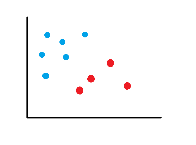
The SVM will choose a hyperplane to separate the groups, with the greatest possible distance:

A good margin is one in which you have the maximum distance from the support vectors to the two classes.

When the data set is more complex, the SVM converts the data into a linear space using some equations to reach a higher dimensional space, use for example: z = x² + and²

Support Vector Regression

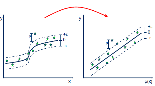
Support Vector Regression uses the same principle with some minor changes. In principle, since the output is a real number, it becomes difficult to predict the information by hand since there are infinite possibilities. For the case of regression, then a margin of tolerance (epsilon) is established near the vector in order to minimize the error taking into account that part of that error is tolerated.

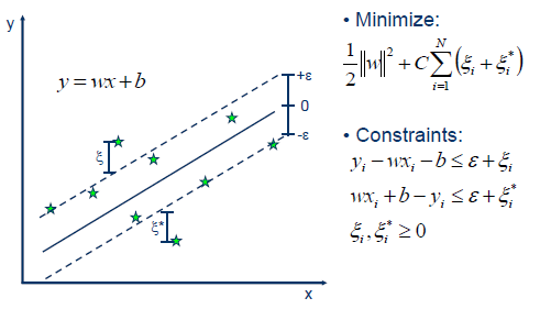
In the case of a linear problem, the SVR is given by

When the problem is not linear, the Kernel function transforms the data into a higher dimensional space characteristic to make it possible to perform the linear separation:

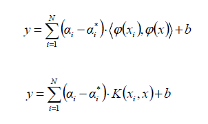
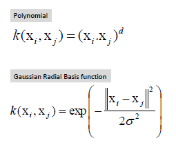
The most common Kernel functions are:

SVR - Support Vector Regression with Python

We import the basic libraries and load the set of data that we will use for this example:

import numpy ace np
import matplotlib.pyplot ace plt
import pandas ace pd dataset = pd.read_csv ('Salario_por_Posicion.csv') X = dataset.iloc [:, 1:2] .values ​​y = dataset.iloc [:, 2] .values

The data set contains 3 columns, of which we will use the second column that represents the level of a person's position, as the independent variable and the salary that is the last column as the dependent variable to predict

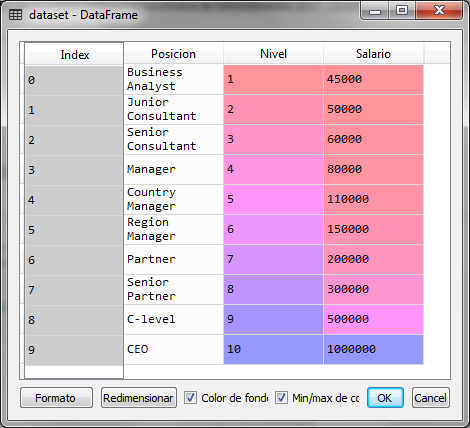
Now we make a scale adjustment through data standardization:

# Scale settings
desde sklearn.preprocessing import StandardScaler sc_X = StandardScaler () sc_y = StandardScaler () X = sc_X.fit_transform (X) y = sc_y.fit_transform (y)

The data is now as follows for the independent variable X and the dependent variable Y

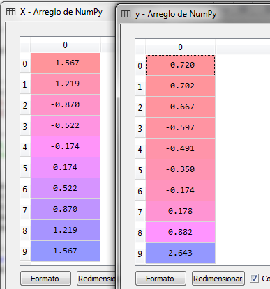
The next step is to create the SVR object from the sklearn library and the SVM subpackage to train it with the X and Y data using the RBF kernel function

desde sklearn.svm import SVR regressor = SVR (kernel = 'rbf') regressor.fit (X, y)

The output obtained after executing the previous block is:

SVR (C = 1.0, cache_size = 200, coef0 = 0.0, degree = 3, epsilon = 0.1, gamma = 'auto', kernel = 'rbf', max_iter = -1, shrinking = True, tol = 0.001, verbose = False )

Para las funciones kernel tenemos varias opciones: linear, poly, rbf, sigmoid o precomputed. la funcion rbf es la función de base radial comúnmente utilizada para  el entrenamiento de algoritmos.

Now with the trained model, we can make a prediction, for the value of X (Level), for example 6.5, for this we first transform the value with the StandarScaler object and send it to the predict method (), the result is transformed in reverse to obtain the value of the calculated salary:

# prediction of a new value
x_trans = sc_X.transform ([[6.5]]) y_pred = regressor.predict (x_trans) y_pred = sc_y.inverse_transform (y_pred)

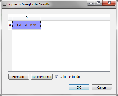
The value of y_pred is 170,370.02 which is the salary calculated for level 6.5, we observe in the original table that the salary for level 6 is 150,000 and for level 7 it is 200,000, so the value of 170 thousand is in the prediction space

Now we graph the real values ​​of x and Y with red and the line of the prediction with blue to observe the curve and the values ​​calculated with the prediction of the SVR

#Graficando the real values
x_real = sc_X.inverse_transform (X) y_real = sc_y.inverse_transform (y) X_grid = np.arange (min (x_real), max (x_real), 0.01) X_grid = X_grid.reshape ((len (X_grid), 1)) x_grid_transform = sc_X.transform (X_grid) y_grid = regressor.predict (x_grid_transform) y_grid_real = sc_y.inverse_transform (y_grid) plt.scatter (x_real, y_real, color = 'net') plt.plot (X_grid, y_grid_real, color = 'blue') plt.title ('SVR') plt.xlabel ('Salary Level') plt.ylabel ('Salary') plt.show ()

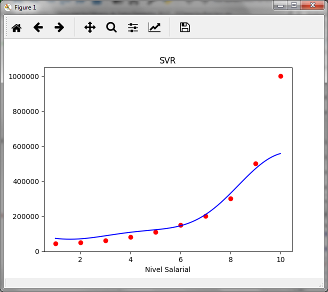
You can compare the result with what is shown in the article on regression trees and observe the difference, in this case it is not a classification to assign the value to a group, but an interpolation.