Linear Regression with Python
Introduction to Linear Regression
The linear regression is one of the analytical or inference methods, where some of the variables stand out as main dependent in relation to the rest of the variables, that is, the dependent variable is defined or explained by the others independent variables.
The relationship that exists between the dependent variable and the independent variables could be linked to a possible equation or model that links them, mainly when all the variables are quantitative. In this way, you can reach predict the value of the dependent variable knowing the profile of all the others.
If the dependent variable is qualitative dichotomous, that is, (0, 1) or (Yes, No), then the linear regression could be used as sorter. If the qualitative dependent variable confirms the assignment of each element in previously defined groups, two or more, it can be used to classify new cases and convert it into the discriminant analysis.
On the other hand, if the dependent variable is qualitative and the independent variables are quantitative, it is a model of variance analysis. But if the dependent variable is qualitative or quantitative and the independent variables are qualitative, then it is a case of segmentation.
In the linear regression both the independent variables and the dependent variable are quantitative and the linear model is given by the equation:
Where b1, b2, ... bn are the coefficients or parameters that denote the magnitude of the effect that the independent variables x1, x2, ... xn have on the independent variable y.
The coefficient b0 is the constant term oo independent of the model. yu is the term that represents the model error.
Ahora, si se dispone de un conjunto de observaciones para cada una de las variables independientes y dependiente, ¿Cómo podemos entonces conocer los valores numéricos de los parámetros b0, b1, .. bn basados en los datos de las variables? Esto es conocido como estimación de los parámetros del modelo y una vez obtenidos estos valores, se podrá realizar una prediction of the future behavior of the variable y.
For example, if we have a hypothetical case where we create a table with information about sales in past periods, based on the advertising expense, the number of interested prospects and the number of quotes made in each period, we could infer sales for later periods:
| Prospects | Advertising | Quotes | Sales |
| 300 | 5,000.00 | 100 | 50,000.00 |
| 400 | 4,500.00 | 120 | 45,000.00 |
| 200 | 7,000.00 | 90 | 30,000.00 |
| 800 | 7,000.00 | 350 | 90,000.00 |
| 600 | 7,500.00 | 220 | 75,000.00 |
| 650 | 4,800.00 | 300 | 81,000.00 |
| 180 | 3,000.00 | 100 | 28,000.00 |
| 700 | 6,500.00 | 400 | 128,000.00 |
| 700 | 5,400.00 | 300 | 89,000.00 |
Prospects (x1), advertising (x2) and quotes (x3) are the independent variables of 9 cases and sales is the dependent variable of those same 9 cases or observations.
Using the linear regression we could calculate the sales that would be had if there were 900 prospects, an advertising expense of 10,000 and the realization of 500 quotes. For this we could apply the model, so it would be necessary to know what the values of the parameters b1, b2 and b3 are mainly.
Simple Linear Regression
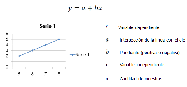
In the case of simple linear regression, the model would only have one coefficient, since there would only be one independent variable, as in the following equation:

where i = 1 .. n and n is the total of cases or observations
when we clear b0 we have the equation:

where Y(average) is the average value of the dependent variable for all cases and x(average) is the average of the values of the independent variable for all cases
When clearing b1 for all cases we have that the value of b1 is given by:

Once the coefficients of the equation have been calculated, we can calculate y for new values of x with which we will be making a prediction.
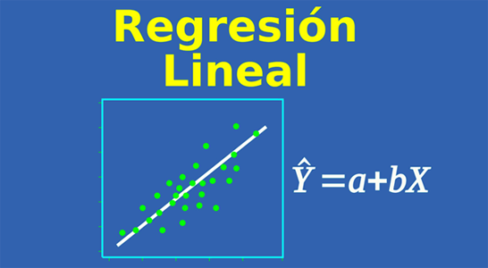
In summary, simple linear regression can be seen as follows:
We can calculate any value of y for values of x that are not in the current data set and that we use as a training set, that is, for the calculation of the coefficients of the equation.
Python
For the example with python, let's consider the following data table:
| Years of experience | Salary |
| 1.1 | 39,343.00 |
| 1.3 | 46,205.00 |
| 1.5 | 37,731.00 |
| 2 | 43,525.00 |
| 2.2 | 39,891.00 |
| 2.9 | 56,642.00 |
| 3 | 60,150.00 |
| 3.2 | 54,445.00 |
| 3.2 | 64,445.00 |
| 3.7 | 57,189.00 |
| 3.9 | 63,218.00 |
| 4 | 55,794.00 |
| 4 | 56,957.00 |
| 4.1 | 57,081.00 |
| 4.5 | 61,111.00 |
| 4.9 | 67,938.00 |
| 5.1 | 66,029.00 |
| 5.3 | 83,088.00 |
| 5.9 | 81,363.00 |
| 6 | 93,940.00 |
| 6.8 | 91,738.00 |
| 7.1 | 98,273.00 |
| 7.9 | 101,302.00 |
| 8.2 | 113,812.00 |
| 8.7 | 109,431.00 |
| 9 | 105,582.00 |
| 9.5 | 116,969.00 |
| 9.6 | 112,635.00 |
| 10.3 | 122,391.00 |
| 10.5 | 121,872.00 |
Where the independent variable X represents the years of experience and the dependent variable AND the salary. We save this data in a text file separated by commas as CSV using Excel and we give it the name Salary_Data.csv
The first thing we will do is import the libraries that we are going to require:
# Simple Linear Retraction
import numpy ace np
import matplotlib.pyplot ace plt
import pandas ace P.S
numpy is a fundamental package for scientific computation with python because it contains objects and functions to perform operations with multidimensional arrays, tools to integrate fortran code and C / C ++, support for linear algebra, Fourier transform and the ability to generate numbers random.
matplotlib contains the tools, functions and objects to create graphics
pandas is the library to manipulate data structures, it is an extension of numpy that also allows the manipulation of external data files.
So the next step is to load the Salary_Data.csv file using the pandas library and separate the dependent and independent variables:
# Simple Linear Retraction import numpy ace np import matplotlib.pyplot ace plt import pandas ace P.S # We load the data set dataset = pd.read_csv ('Salary_Data.csv') x = dataset.iloc [:,:-1] .values y = dataset.iloc [:, 1] .values
Once the independent and dependent variables are created with the data of years of experience and salary, we will divide both vectors into two vectors each. The first one with random data extracted from the independent variable (years of experience) to create a set of data to train the model, that is, to calculate the coefficients a and b (or b0 and b1), which we call the training set and the second to test the model, so we call it the test set.
# Simple Linear Retraction import numpy ace np import matplotlib.pyplot ace plt import pandas ace P.S # We load the data set dataset = pd.read_csv ('Salary_Data.csv') x = dataset.iloc [:,:-1] .values y = dataset.iloc [:, 1] .values # We divide the data into the training set and the test set desde sklearn.cross_validation import train_test_split x_train, x_test, y_train, y_test = train_test_split (x, y, test_size =1/3, random_state =0)
From the Sci-Kit Learn (sklearn) library we import the function train_test_split to divide the data. In the function we use the variables x and y plus two additional parameters: test_size and random_state. With the first one (test_size) we indicate that the size for the test set, stored in the variables x_test and y_test, will have a third of the total set, ie 10 records, given that the total set is 30 and the 10 selected will be chosen from randomly from among those 30, since the last parameter of the function is random_state = 0.
The next step is to load the training set to the linear regression model to calculate the coefficients, that is, to train the model.
# Simple Linear Retraction import numpy ace np import matplotlib.pyplot ace plt import pandas ace P.S # We load the data set dataset = pd.read_csv ('Salary_Data.csv') x = dataset.iloc [:,:-1] .values y = dataset.iloc [:, 1] .values # We divide the data into the training set and the test set desde sklearn.cross_validation import train_test_split x_train, x_test, y_train, y_test = train_test_split (x, y, test_size =1/3, random_state =0) # We load the training set to the Linear Regression model desde sklearn.linear_model import LinearRegression regressor = LinearRegression () regresor.fit (x_train, y_train)
From the same library sklearn in the subpackage linear_model we import the class LinearRegression and create the object regressor with the constructor of the class.
Once the object is created, we invoke the fit () method by providing the training data.
Now with the trained model, we can now predict the values of Y with the test set x_test and compare with the real values y_test.
# Simple Linear Retraction import numpy ace np import matplotlib.pyplot ace plt import pandas ace P.S # We load the data set dataset = pd.read_csv ('Salary_Data.csv') x = dataset.iloc [:,:-1] .values y = dataset.iloc [:, 1] .values # We divide the data into the training set and the test set desde sklearn.cross_validation import train_test_split x_train, x_test, y_train, y_test = train_test_split (x, y, test_size =1/3, random_state =0) # We load the training set to the Linear Regression model desde sklearn.linear_model import LinearRegression regressor = LinearRegression () regressor.fit (x_train, y_train) # Prediction of the results of the test suite (x_test) y_pred = regressor.predict (x_test) #Now we compare y_pred with the real values y_test
Now that we have the values calculated with the linear regression model, we can compare them against the real values (y_pred vs y_test) by showing a graph.
# Simple Linear Retraction import numpy ace np import matplotlib.pyplot ace plt import pandas ace P.S # We load the data set dataset = pd.read_csv ('Salary_Data.csv') x = dataset.iloc [:,:-1] .values y = dataset.iloc [:, 1] .values # We divide the data into the training set and the test set desde sklearn.cross_validation import train_test_split x_train, x_test, y_train, y_test = train_test_split (x, y, test_size =1/3, random_state =0) # We load the training set to the Linear Regression model desde sklearn.linear_model import LinearRegression regressor = LinearRegression () regressor.fit (x_train, y_train) # Prediction of the results of the test suite (x_test) y_pred = regressor.predict (x_test) #Now we compare y_pred with the real values y_test plt.scatter (x_test, y_test, color = 'net') plt.plot (x_train, y_pred, color = 'blue') plt.title ('Salary vs. Experience (Trial Set)') plt.xlabel ('Years of experience') plt.ylabel ('Salary') plt.show ()
With red dots the real values for Y of the test set are shown and the blue line shows the regression line calculated for the predicted values.
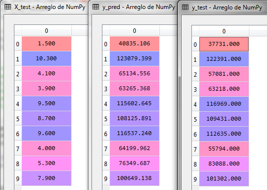
The values of both vectors are the following:

The table on the left side shows the years of experience (x_test), for the 10 values of the test set, the table in the middle y_test is the original salary corresponding to the years of experience. The table on the far right shows the values calculated with the linear regression model for the salary corresponding to years of experience.
For example, in the second line mentions that with 10.3 years of experience the current salary is 123,079.39 and the prediction indicates a salary of 122,391.00 the difference is 688.39
We can see that the values are different, but not very far from reality. The error is minimal and the result of the regression can be accepted for unknown values of x.
recommendations
To start with the programming in python, this course of Introduction to programming with python It can be very useful. On the other hand, in this webinar you will be able to know the architectural details and solutions for Azure machine learning.
Also for the development in the cloud we can use Amazon Web Services, these leagues are for the certification course of Associated and the one Professional in AWS design and architecture.


Wow, it seems interesting how can code solve those problems. What method should we use?
Hello, that's an interesting topic to discuss. Agree with an innovation that you share through this article. Could I add some points?
Hello, you can use object oriented programming as well
Sure, what points would you add?
Muy buen ejemplo, bien explicado
Quisiera saber como poder aplicar regresion lineal para predecir la disponibilidad de playas de estacionamiento conociendo las entradas y salidas? o se necesitarian mas variables?
Hola Alex,
Que variables estas considerando? únicamente fecha y hora de entrada y salida?
Que esas variables podrías hacer la prueba, pero talvez en este caso requieras series de tiempo
Muchas Gracias, Saludos!!!
Hola! he modificado un poco tu codigo pero a la hora de graficar obtengo un error al nombrar los ejes, obtengo el siguiente error: TypeError: ‘str’ object is not callable Aqui esta el codigo completo, como podria resolver este error? te agradezco por el ejemplo y tu ayuda, saludos, Jesus import numpy as np import matplotlib.pyplot as plt import pandas as pd dataset = pd.read_csv(‘/Users/jesusjm/Data science Phyton/Salary_Data.csv’) type(dataset) dataset.head() x = dataset.iloc[:, :-1].values y = dataset.iloc[:, 1].values y from sklearn.linear_model import LinearRegression regressor = LinearRegression() regressor.fit(x, y) print(f’intercepto ‘,regressor.intercept_) print(f’pendientes ‘,regressor.coef_) ypred = regressor.predict(x) plt.scatter(x,y) plt.plot(x,ypred, color=”darkorange”) plt.title(‘hola’) plt.xlabel(‘Años... Read more »
Hola! ya resolvi el problema! gracias!
Excelente
Hola Jesús,
Perdón por la tardanza en responder, pero veo que si pudiste resolverlo. Saludos