Linear Discriminant Analysis
The discriminant analysis is a predictive technique of ad hoc classification and is so named because groups or classes are previously known before making the classification, which unlike decision trees (post hoc) where the classification groups are derived from the execution of the same technique without knowing previously.
Siquieres verlo en video:
It is an ideal technique to build a predictive model and forecast the group or class to which an observation belongs based on certain characteristics that define its profile.
As the name implies, discriminant analysis helps identify the characteristics that differentiate (discriminate) to two or more groups and to create a function capable of distinguishing, as accurately as possible, the members of one group or another.
On the other hand, LDA It is also a method of dimension reduction, given that taking n variables independent of the data set, the estrae method p <= n new independent variables that contribute most to class separation of the dependent variable.
The interpretation of the differences between groups is to determine:
- To what extent a set of characteristics allows us to extract dimensions that differentiate groups and
- Which of these characteristics are those that contribute the most to such dimensions, that is, which have the greatest power of discrimination.
In summary, we can say that Linear Discriminant Analysis - LDA has the following applications:
- It is widely used as a dimension reduction technique
- It is used as a step in the pre-processing of data for the classification of patterns
- Its objective is to project a data set in a smaller space
The objective of the LDA is to project the space of a characteristic (data set of n dimensions) in a small subspace k where k <= n - 1, maintaining the discriminatory information of classes.
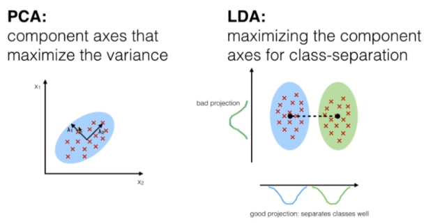
Both PCA (Principal Component Analysis) and LDA (Linear Discriminant Analysis) are linear transformation techniques used for dimension reduction, however, PCA is unsupervised and LDA is supervised given its relationship with the dependent variable.
The 5 general steps for linear discriminant analysis are:
- Calculate the mean vectors d-dimensional for the different classes of the data set.
- Calculate scatter matrices (between classes and within classes).
- Calculate the eigenvectors (e1, e2, ... ed) and their corresponding eigenvalues (l1, l2, ..., ld) for the dispersion matrices
- Sort the eigenvectors in a decreasing way in relation to the eigenvalues and select the k eigenvectors with the largest eigenvalues to form a dimension matrix dxk called W (where each column represents an eigenvector).
- Use the dxk matrix of eigenvectors to transform the samples into a new sub space. This can be summarized by the multiplication of matrices Y = X x W (where X is a nxd matrix that represents the n samples and y is the nxk transform of the samples in the new sub space).
If the objective is to reduce the dimension of a d-dimensional data set to project it in a k-dimensional sub space (where k ˂ d), how to know what size to select for k (where k is the number or dimension of the new sub space) and how to know if we have a sub space that correctly represents the data.
Calculate the eigenvectors for the data set and concentrate them to form the scattering matrices, where each of these vectors is associated with an eigenvalue which indicates the size or magnitude of the vectors.
If we observe that all eigenvalues have similar magnitudes, then this is a good indicator that the data is already projected to a good sub space.
But, if one of the eigenvalues is much larger than others, what is interesting is to keep only those vectors that have the largest eigenvalues, since they contain more information related to the distribution of the data. Values that are closer to zero are less informative and should not be taken for the creation of the new sub space.
Implementation of LDA with Python
For the exercise with python we will consider a data set with characteristics of three wine categories. The characteristics are conformed with 13 variables that go from the degree of alcohol, the acidity, the aroma, etc. To form three customer segments that represent the classes or groups. In total there are 179 records or samples.
| Alcohol | Malic Acid | Ash | Ash Alcanity | Magnesium | Total Phenols | Flavanoids | Nonflavanoid Phenols | Proanthocyanins | Color_Intensity | Hue | OD280 | Proline | Customer Segment |
| 14.23 | 1.71 | 2.43 | 15.6 | 127 | 2.8 | 3.06 | 0.28 | 2.29 | 5.64 | 1.04 | 3.92 | 1065 | 1 |
| 13.2 | 1.78 | 2.14 | 11.2 | 100 | 2.65 | 2.76 | 0.26 | 1.28 | 4.38 | 1.05 | 3.4 | 1050 | 1 |
| 13.16 | 2.36 | 2.67 | 18.6 | 101 | 2.8 | 3.24 | 0.3 | 2.81 | 5.68 | 1.03 | 3.17 | 1185 | 1 |
| 14.37 | 1.95 | 2.5 | 16.8 | 113 | 3.85 | 3.49 | 0.24 | 2.18 | 7.8 | 0.86 | 3.45 | 1480 | 1 |
| 13.24 | 2.59 | 2.87 | 21 | 118 | 2.8 | 2.69 | 0.39 | 1.82 | 4.32 | 1.04 | 2.93 | 735 | 1 |
| 14.2 | 1.76 | 2.45 | 15.2 | 112 | 3.27 | 3.39 | 0.34 | 1.97 | 6.75 | 1.05 | 2.85 | 1450 | 1 |
| 14.39 | 1.87 | 2.45 | 14.6 | 96 | 2.5 | 2.52 | 0.3 | 1.98 | 5.25 | 1.02 | 3.58 | 1290 | 1 |
| 14.06 | 2.15 | 2.61 | 17.6 | 121 | 2.6 | 2.51 | 0.31 | 1.25 | 5.05 | 1.06 | 3.58 | 1295 | 1 |
| 14.83 | 1.64 | 2.17 | 14 | 97 | 2.8 | 2.98 | 0.29 | 1.98 | 5.2 | 1.08 | 2.85 | 1045 | 1 |
| 13.86 | 1.35 | 2.27 | 16 | 98 | 2.98 | 3.15 | 0.22 | 1.85 | 7.22 | 1.01 | 3.55 | 1045 | 1 |
| 14.1 | 2.16 | 2.3 | 18 | 105 | 2.95 | 3.32 | 0.22 | 2.38 | 5.75 | 1.25 | 3.17 | 1510 | 1 |
| 14.12 | 1.48 | 2.32 | 16.8 | 95 | 2.2 | 2.43 | 0.26 | 1.57 | 5 | 1.17 | 2.82 | 1280 | 1 |
| 13.75 | 1.73 | 2.41 | 16 | 89 | 2.6 | 2.76 | 0.29 | 1.81 | 5.6 | 1.15 | 2.9 | 1320 | 1 |
| 14.75 | 1.73 | 2.39 | 11.4 | 91 | 3.1 | 3.69 | 0.43 | 2.81 | 5.4 | 1.25 | 2.73 | 1150 | 1 |
To start with the model, we load the file with the data and we separate in X the independent variable columns 1 to 13 and in Y the dependent variable column 14 with the customer segmentation.
# LDA # Import of libraries import numpy ace np import matplotlib.pyplot ace plt import pandas ace P.S # Importation of the dataset dataset = pd.read_csv ('Vinos.csv') X = dataset.iloc [:, 0:13] .values y = dataset.iloc [:, 13] .values
We divided the data set into a training set and a set of tests to train the LDA model, then we made a scale adjustment and we created the LDA model to reduce the dimension to 2 variables.
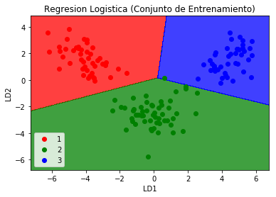
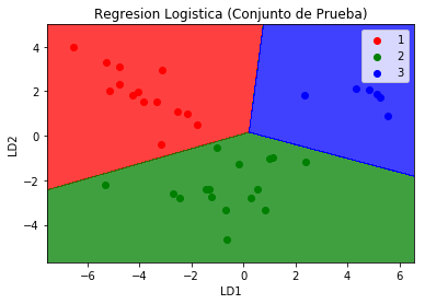
To prove that with 2 of 13 variables we can make a prediction or classification of the 3 groups of wines, we use the logistic regression and check the confusion matrix
# Import of libraries
import numpy ace np
import matplotlib.pyplot ace plt
import pandas ace P.S
# Importation of the dataset
dataset = P.S.read_csv('Vinos.csv')
X = dataset.iloc[:, 0:13].values
Y = dataset.iloc[:, 13].values
# We divide the data set into training sample and
# test sample
desde sklearn.model_selection import train_test_split
X_train, X_test, y_train, y_test = train_test_split(X, Y,
                                                    test_size = 0.2,
                                                    random_state = 0)
# Adjustment of Scales
desde sklearn.preprocessing import StandardScaler
sc = StandardScaler()
X_train = sc.fit_transform(X_train)
X_test = sc.transform(X_test)
# Applying LDA
desde sklearn.discriminant_analysis import LinearDiscriminantAnalysis ace LDA
lda = LDA(n_components = 2)
X_train = lda.fit_transform(X_train, y_train)
X_test = lda.transform(X_test)
# We check the resulting independent variables with
# a Logistic regression to determine that with only two
# variables we get the right prediction
desde sklearn.linear_model import LogisticRegression
classifier = LogisticRegression(random_state = 0)
classifier.fit(X_train, y_train)
# Prediction of the test set for
# buy the results
y_pred = classifier.predict(X_test)
# We create the confusion matrix
desde sklearn.metrics import confusion_matrix
cm = confusion_matrix(y_test, y_pred)
# Visualization of training data
desde matplotlib.colors import ListedColormap
X_set, y_set = X_train, y_train
X1, X2 = np.meshgrid(np.arange(start = X_set[:, 0].min() - 1, stop = X_set[:, 0].max() + 1, step = 0.01),
                     np.arange(start = X_set[:, 1].min() - 1, stop = X_set[:, 1].max() + 1, step = 0.01))
plt.contourf(X1, X2, classifier.predict(np.array([X1.ravel(), X2.ravel()]).T).reshape(X1.shape),
             alpha = 0.75, cmap = ListedColormap(('net', 'green', 'blue')))
plt.xlim(X1.min(), X1.max())
plt.ylim(X2.min(), X2.max())
for i, j in enumerate(np.unique(y_set)):
    plt.scatter(X_set[y_set == j, 0], X_set[y_set == j, 1],
                c = ListedColormap(('net', 'green', 'blue'))(i), label = j)
plt.title('Logistic Regression (Training Set)')
plt.xlabel('LD1')
plt.ylabel('LD2')
plt.legend()
plt.Show()
# Visualization of the test results
desde matplotlib.colors import ListedColormap
X_set, y_set = X_test, y_test
X1, X2 = np.meshgrid(np.arange(start = X_set[:, 0].min() - 1, stop = X_set[:, 0].max() + 1, step = 0.01),
                     np.arange(start = X_set[:, 1].min() - 1, stop = X_set[:, 1].max() + 1, step = 0.01))
plt.contourf(X1, X2, classifier.predict(np.array([X1.ravel(), X2.ravel()]).T).reshape(X1.shape),
             alpha = 0.75, cmap = ListedColormap(('net', 'green', 'blue')))
plt.xlim(X1.min(), X1.max())
plt.ylim(X2.min(), X2.max())
for i, j in enumerate(np.unique(y_set)):
    plt.scatter(X_set[y_set == j, 0], X_set[y_set == j, 1],
                c = ListedColormap(('net', 'green', 'blue'))(i), label = j)
plt.title('Logistic Regression (Test Set)')
plt.xlabel('LD1')
plt.ylabel('LD2')
plt.legend()
plt.Show()
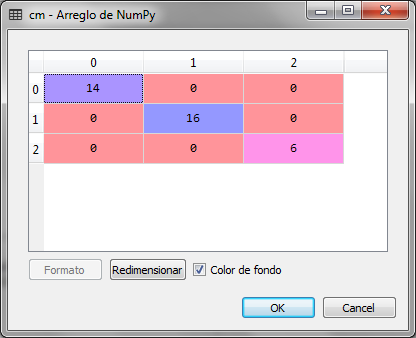
We observed that the confusion matrix for the prediction of the group with the logistic regression for the new variables with the reduced dimension is very accurate and there are no errors
hello hello, your explanation is very good, I am doing an exercise using scikit learn but the data I am using are only two variables with 4 classes and using the discriminant linear analysis algorithm, could you help me?
Hello John,
I'm sorry for answering delay.
Yes, with pleasure, what do you need?