Análisis del Componente Principal PCA

Principal Component Analysis

The PCA is a tool for reduce dimensionality in the data that can be used to convert a fairly large set of variables into a smaller set that contains the largest amount of information contained in the large set.

Si quieres verlo en video:

In this sense, the PCA is a mathematical procedure that transforms a set of correlated variables into a set (smaller) of variables not correlated calls main components.

The first principal component represents the greatest possible amount of variability in the data and each subsequent component explains most of the remaining variability, ie, that the smallest data set should preserve the variance of the original data.

For example, a two-dimensional data set can be reduced by projecting points on a line, so each instance in the data set can be represented by a single value instead of a pair of values. A three-dimensional data set can be reduced to two dimensions by projecting the variables in a plane.

In general, a set of n dimensions it can be reduced by projecting the data set into a subspace of k dimensions, where k is less than n.

More formally, PCA can be used to find a set of vectors spanning a subspace, which minimizes the sum of the quadratic error of the projected data. The projection will retain the largest proportion of the variance of the original data.

PCA rotates the data set to align it with its main components to maximize the variance contained within the first major components. Suppose we have the following set of data plotted in the figure:

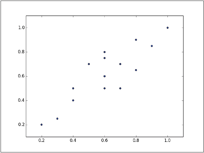
The instances form an approximate ellipse that can be seen from the origin to the top right of the graph. To reduce the dimension of this data set, we must project the points in a line. The following graph shows two lines where the data could be projected. In each of them, the variance is different, so the task is to see in which of the two lines the instances have the greatest variation.

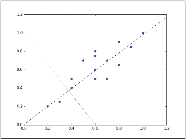
Lines on which the data of the set can be projected

Instances have the most variation on the dashed line, rather than on the dotted line. In fact, the line in dashes is the first main component. The second main component must be orthogonal to the first, that is, that the second main component must be statistically independent, and apparently it will be perpendicular to the first main component, as shown in the following figure:

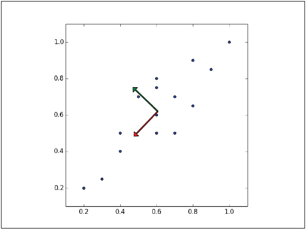
Each subsequent principal component preserves the greater amount of the remaining variance, the only restriction being that each must be orthogonal to the previous one.

If we now consider that the data has three variables, so the data set is three-dimensional:

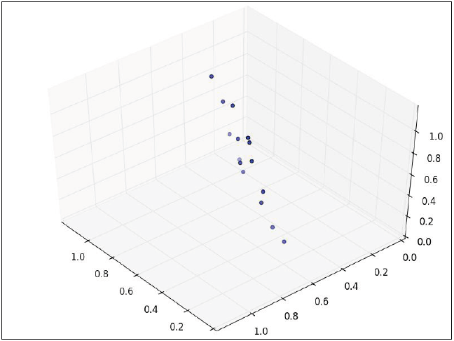
The points can be rotated and moved in such a way that two dimensions are accommodated and the points now form an ellipse, the third dimension has almost no variance and then it can be discarded.

The PCA is most useful when the variance in the data set is unevenly distributed along the dimensions. If, on the contrary, a data set between three dimensions forms a convex sphere, the PCA analysis could not be as effective since there is a similar variance in each dimension, none of the dimensions can be discarded without losing significant information.

Visually it is easier to identify the main components when the data set is composed of only two or three dimensions. For a larger dimension set the calculations for the main components are described in the following sections.

Variance and Covariance

Before entering fully with the calculations to identify the main components, let's see some basic concepts.

Variance

The variance is the measure that tells us how scattered or distributed a set of values is. The variance is calculated as the average of the square of the difference in values with respect to the average of that set of values:

Covariance

Covariance is the measure of how much two variables change together. It is a measure of the strength of the correlation between two sets of variables. If the covariance between two variables is zero, variables They're not here correlated. However, the fact that two variables are not correlated does not imply that they are independent, since the correlation is only a measure of linear dependence and is calculated with the following equation:

If the covariance is not zero, the sign indicates whether the variables are positive or negatively correlated. If two variables are positively correlated, it means that one increases its value when the other increases it.

When two variables are negatively correlated means that a variable has a decrease relative to its mean when the other variable presents an increase relative to its mean.

The covariance matrix describes the values of the covariance between each pair of values in the data set. The element (i, j) indicates the covariance of the dimension i, j of the data. For example, the covariance matrix of a three-dimensional data set would look like this:

Covariance matrix of a 3-dimensional set

If as an example we consider the following data set:

2	0	-1.4
2.2	0.2	-1.5
2.4	0.1	-1
1.9	0	-1.2

In the previous table we have 3 variables as 4 cases, then the average of each variable is: 2.125, 0.075 and -1.275, with this we can now calculate the covariance of each pair of variables to generate the following covariance matrix.

Covariance matrix of the previous data set

Using Numpy we can generate the covariance matrix in the following way:

import numpy ace np X = [[2, 0, -1.4], [2.2, 0.2, -1.5], [2.4, 0.1, -1], [1.9, 0, -1.2]] print np.cov (np.array (X ) .T out: [[0.04916667 0.01416667 0.01916667] [0.01416667 0.00916667 -0.00583333] [0.01916667 -0.00583333 0.04916667]]

Own and Own Values

A vector is described by its direction and its magnitude, or length. An eigenvector of a matrix is a nonzero vector that satisfies the following equation:

In the previous equation v is the own vector TO is a square matrix and lanbda it is a scalar called own value. The direction of the eigenvector remains the same after being transformed by A, only its magnitude changes, given by the eigenvalue, that is to say that multiplying a matrix by one of its eigenvectors is equivalent to scaling the eigenvector.

In English a vector of its own is known as eigenvector and the word eigen in German means belongs to, or that is peculiar to, so that the eigenvector of a matrix is a vector that belongs to, and characterizes the structure of the data.

Both the eigenvectors and the eigenvalues can only be derived from square matrices and not all square matrices have eigenvectors or eigenvalues. If a matrix has vectors and eigenvalues, it will have a pair for each of its dimensions. The main components of a matrix are the eigenvectors of its covariance matrix, ordered by their corresponding eigenvalues.

The eigenvector with the largest eigenvalue is the first main component, the second main component is the eigenvector with the second largest eigenvalue and so on.

As an example, let us calculate the eigenvectors and their eigenvalues of the following square matrix:

From the equation we showed previously, remember that the product of the matrix A and any of its eigenvectors must be equal to the eigenvector multiplied by its eigenvalue.

Let's start by finding the eigenvalues, which can be found with the following characteristic equations:

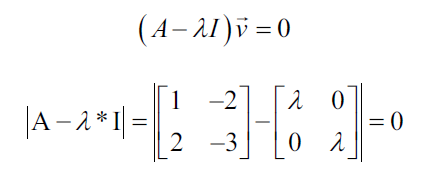
The characteristic equation states that the determinant of the matrix, that is, the difference between the data of the matrix and the product of the identity matrix and an eigenvalue is zero:

Both eigenvalues of this matrix are equal to -1. So now we can use the eigenvalues to solve the eigenvectors

First, we make the equation equal to zero:

Substituting the values for A we have the following:

Now we can substitute the first eigenvalue to solve the eigenvectors.

Now we show the resulting equations as a system of equations:

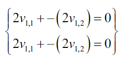
Each nonzero vector that satisfies the previous equations, can be used as own vector:

PCA requires unit vectors or vectors that have a length of 1, so you can normalize the vectors by dividing them by their normal, which is achieved with the following equation:

The norm of the vector is the following:

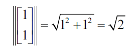
This generates the following unitary own vector:

To verify with Numpy that the previous solution is correct, we can do the following where the eig function returns a tuple of eigenvalues and the eigenvectors.

import numpy ace np v, w = np.linalg.eig (np.array ([[1, -2], [2, -3]])) w; v arrray ([- 0.99999998, -1.00000002]) array ([[0.70710678, 0.70710678], [0.70710678, 0.70710678]])

Reduction of Dimensionality

Using PCA (Principal Component Analysis) to reduce the following two-dimensional data set in only one dimension:

x1	x2
0.9	1
2.4	2.6
1.2	1.7
0.5	0.7
0.3	0.7
1.8	1.4
0.5	0.6
0.3	0.6
2.5	2.6
1.3	1.1

The first step is to subtract the mean of each variable in each of the cases

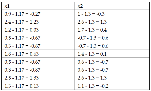
Now we calculate the main components of the data. Recalling that the principal components are the eigenvectors of the covariance matrix ordered by the eigenvalues.

The main components can be found using two different techniques. The first technique requires calculating the covariance matrix of the data. Since the covariance matrix will be a square matrix, we can calculate the vectors and eigenvalues as described above.

The second technique uses the decomposition of the singular value of the data matrix to find the vectors and the square root of the eigenvalues of the covariance matrix. We use the first technique to describe the process and the second technique with the library scikit-learn.

The following matrix is the covariance matrix of the data

Using the technique described above, the eigenvalues are 1,250 and 0.034. The following matrix represents the unit eigenvectors:

Now we project the data into the main components. The first eigenvector has the highest eigenvalues and is the first principal component. We build a transformation matrix where each column of the matrix is the proper vector for a main component.

If you were reducing a 5-dimensional data set in a three-dimensional set, you would build a transformation matrix with 3 columns. In this example, we project the two-dimensional data set into one dimension, so we only use the eigenvector for the first principal component.

Finally we calculate the product point of the data matrix with the transformation matrix, resulting in the following:

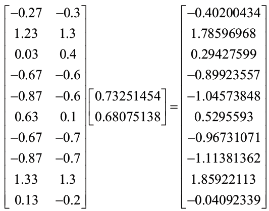
The resulting vector is the resulting dimension, that is, it is the matrix of a dimension that corresponds to the variable that results from reducing the two original dimensions in a dimension of the data set.

PCA with Python

Now we will implement the main component analysis with python, although perhaps before continuing, it might be convenient to review some of the programming course that could help you understand the structure and logic behind the most common languages.

As a first step we import the necessary libraries for machine learning

import numpy ace np
import matplotlib.pyplot ace plt
import pandas ace P.S

For this example we will use a set of data from a wine collection with 13 independent variables and a dependent variable, which gives us the classification of the wine. The independent variables are characteristic values of the wine in question and that go from the alcohol, the aroma, the flavor, the acidity, and other components or ingredients that classify a wine.

# We import the data set
dataset = pd.read_csv ('Wine.csv') X = dataset.iloc [:, 0:13] .values y = dataset.iloc [:, 13] .values

The set of 177 cases with 13 independent variables is as follows:

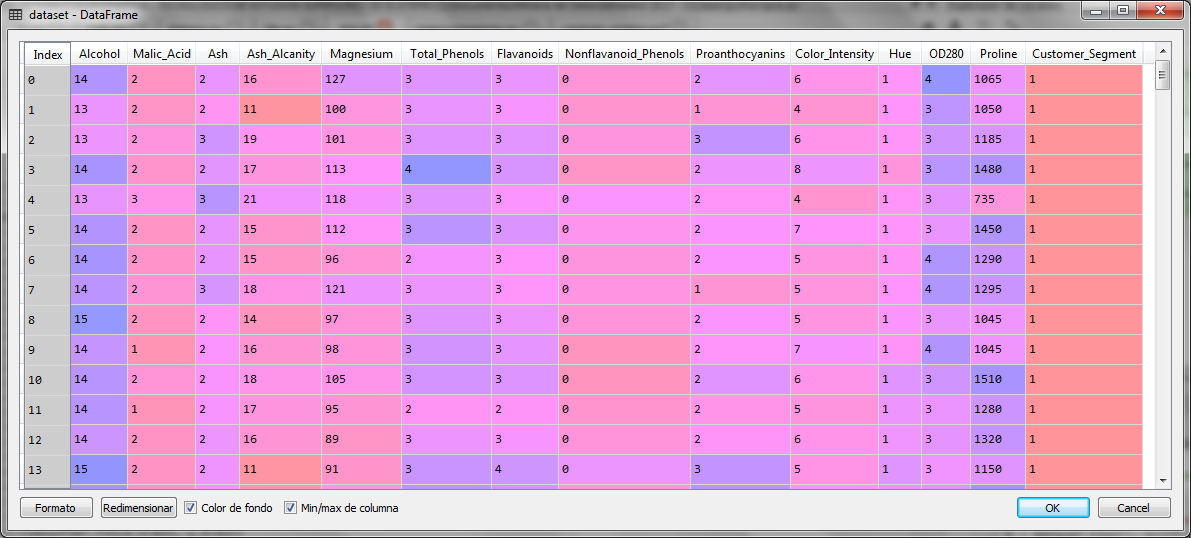
Once we import the data, we separate the independent variables in the X matrix and the dependent variable in the vector y.

Now we divide the data set into two sets for training and testing

# Splitting the dataset into the Training set and Test set
desde sklearn.model_selection import train_test_split X_train, X_test, y_train, y_test = train_test_split (X, y, test_size = 0.2, random_state = 0)

Our next step will be to standardize the scales for the 13 variables

# Feature Scaling
desde sklearn.preprocessing import StandardScaler sc = StandardScaler () X_train = sc.fit_transform (X_train) X_test = sc.transform (X_test)

Once with the normalized data, we apply the PCA to reduce the dimension from 13 to 2 variables.

# Applying PCA
desde sklearn.decomposition import PCA pca = PCA (n_components = 2) X_train = pca.fit_transform (X_train) X_test = pca.transform (X_test)

The training set was now with 2 variables as follows:

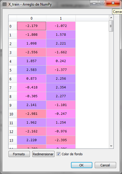
training set reduced from 13 to 2 variables

The same happened with the X_test test set. Now to know how much the variance of the two resulting principal components is expressed, in relation to the original dimension, that is, to the data of the original 13 variables, we can extract that information from the PCA object and analyze it.

# Explanation of the variance # We create a vector with the percentage of influence of the variance # for the two variables resulting from the data set
explained_variance = pca.explained_variance_ratio_

The values of the variable explained_variance are:

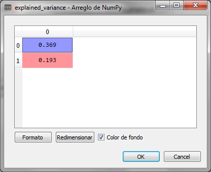
The two resulting principal components are the two eigenvalues of the eigenvectors with the highest value of the original 13 of the data set. From there, the two highest were obtained to obtain the two resulting dimensions or main components. The first represents 36.9% and the second 19.3%

To verify that the two resulting variables represent the original 13 variables, we will make the prediction of the dependent variable with logistic regression, checking the prediction results with the confusion matrix:

# Fitting Logistic Regression to the Training set
desde sklearn.linear_model import LogisticRegression classifier = LogisticRegression (random_state = 0) classifier.fit (X_train, y_train)

# Predicting the Test set results
y_pred = classifier.predict (X_test)

# Making the Confusion Matrix
desde sklearn.metrics import confusion_matrix cm = confusion_matrix (y_test, y_pred)

When making the prediction for the test set, the confusion matrix is as follows:

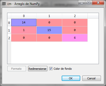
Matrix of confusion of the logistic regression

As observed in the confusion matrix, there is only one error, a false positive in the first of the three classes of wines. So we conclude that the prediction is correct using the data set of two variables, instead of the data set of 13 variables.

Now we can graph the prediction data to observe in a visual way the results of this classification

desde matplotlib.colors import ListedColormap X_set, y_set = X_test, y_test X1, X2 = np.meshgrid (np.arange (start = X_set [:, 0] .min () - 1, stop = X_set [:, 0] .max () + 1, step = 0.01), np.arange (start = X_set [:, 1] .min () - 1, stop = X_set [:, 1] .max () + 1, step = 0.01)) plt.contourf (X1, X2, classifier.predict (np.array ([X1.ravel (), X2.ravel ()]). T) .reshape (X1.shape), alpha = 0.75, cmap = ListedColormap (('net', 'green', 'blue'))) plt.xlim (X1.min (), X1.max ()) plt.ylim (X2.min (), X2.max ()) for i, j in enumerate (np.unique (y_set)) : plt.scatter (X_set [y_set == j, 0], X_set [y_set == j, 1], c = ListedColormap (('net', 'green', 'blue')) (i), label = j) plt.title (' Logistic Regression (Test set) ') plt.xlabel (' PC1 ') plt.ylabel (' PC2 ') plt.legend () plt.show ()

The resulting graph is as follows

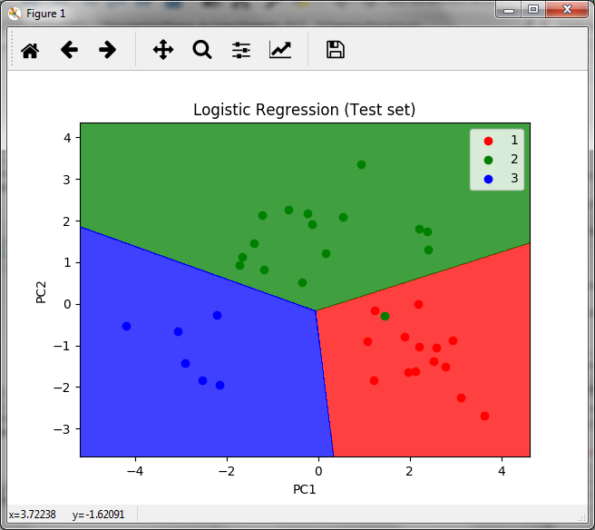
Graph of the prediction with logistic regression

In the graph we observe the areas of the 3 wine classes with the points of the prediction of the test set, where we also observe the only error that exists, the green dot in the red zone.

Final comments

Many times it is necessary to implement this type of examples in the cloud with a greater amount of real data and execute several of the techniques and algorithms of machine learning to make some comparisons with the different classification and / or prediction algorithms. Today there are several providers of resources in the cloud for data science and machine learning, some of them could be: Microsoft Azure, Alibaba Cloud, Amazon Web Services, in this link you can check a webinar to know the different certifications of Azure.

On the other hand, some courses with good discounts for cloud services can be checked in Alibaba, where you can also verify information about the different services.

You can also try the trials without cost for enough time to do all kinds of tests.

Finally, it will always be important to have the foundations of the programming and the management of databases, so here You could find some interesting courses.

If you are interested in the article, share it

5 2 votes

Article Rating