Logistic regression

Logistic regression is a classification method, which unlike simple regression, where a continuous number is predicted, logistic regression is used to predict a category.

The classification has a wide range of applications ranging from medical diagnosis to even marketing. Among the classification models we can talk about linear and non-linear models

Linear classification models

• Logistic regression
• SVM (Support Vector Machine)
• Naive Bayes

Non-linear classification models

• Decision trees
• K-NN (K-Nearest Neighbors)
• Kernel SVM
• Random Forest

When a target variable takes only two values ​​Yes or No, '0' or '1', then the classification problem is known as a binary classification problem and the effective way to deal with this type of problem is to use the Logistic regression.

Normally the linear regression function takes values ​​from a straight line, being this function of the type: f (x) = b₀ + b₁x   and for multiple regression f (x) = b₀ + b₁x₁ + ... + b_nx_n

For the classification problem '0', '1' we can insert   z = m^Tx in the logistic function which is known as the function sigmoid expressed as follows:

The function maps a real number to the interval [0,1] and is used to transform any function of arbitrary value into a function that best fits the classification.

the function f (x) represents the probability P (y = 1 | x; m) so the logistic regression is a type of probabilistic classification used to represent a binary response of a binary predictor.

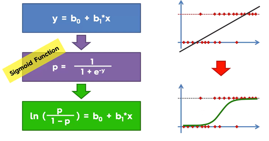
On the curve of the sigmoid function we have the probability value for Y, however for the binary classification, what is required is a decision boundary, which is a curve that separates the area where y = 0 from the area where y = 1 to obtain the classification 0 or 1, so the output of transforms with:

If the estimated value is less than 0.5, the output will be 0 and if the estimated value is greater than or equal to 0.5 then the output of the sigmoid function will be 1.

---

Logistic Regression with Python

For this example of the logistic regression with python we will use a data file that contains information about clients that buy or not certain products online, for this we have information about gender, age and estimated salary, classifying customers with 0 and 1 if you did not buy or if you bought respectively.

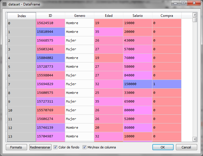
We load the libraries and the data set from the file with:

# Logistic regression

# Import of libraries
import numpy ace np
import matplotlib.pyplot ace plt
import pandas ace P.S

# Importation of the dataset
dataset = pd.read_csv ('Compras_en_Linea.csv') X = dataset.iloc [:, [2, 3]]. values ​​y = dataset.iloc [:, 4] .values

For the independent variable x, we use age and salary, columns 2 and 3, the dependent variable Y is column 4 with information on whether or not it was purchased.

We use 25% of the data contained in the file for tests and 75% for the training set. The complete file contains 400 customer records, so 300 will be used for training and 100 for tests.

# Division of data set in training data # and test data
desde sklearn.cross_validation import train_test_split X_train, X_test, y_train, y_test = train_test_split (X, y, test_size = 0.25, random_state = 0)

Now, given that the value of age and salary are in different scales, we make a scale adjustment with the StandarScaler class

# Scale adjustment
desde sklearn.preprocessing import StandardScaler sc = StandardScaler () X_train = sc.fit_transform (X_train) X_test = sc.transform (X_test)

Now we create the model with the class LogisticRegression from the bookstore sklearn and we train him with the training set data X_train.

# Adjustment of the logistic regression to the training set
desde sklearn.linear_model import LogisticRegression classifier = LogisticRegression (random_state = 0) classifier.fit (X_train, y_train)

Once trained the model we can make the prediction of the data contained in the test set X_test

# Test set prediction
y_pred = classifier.predict (X_test)

y_pred contains the data calculated or predicted by the logistic regression model, so we can buy y_test with y_pred

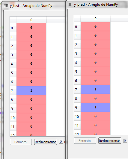
We note that in line 9 there was an error in the prediction, which is why we can generate the confusion matrix to analyze both the false positives and the false negatives.

# Confusion Matrix
from sklearn.metrics import confusion_matrix cm = confusion_matrix (y_test, y_pred)

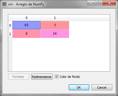
We observe that of the 100 records that the test set contains, 8 records that should be 1 were classified as 0 and 3 records that should be 0 were classified as 1. The results are acceptable, however to achieve better results in the classification we require more data to train the model.

The classification of the customers that belong to the test set is carried out to determine if the customer buys or does not buy. This set contains unknown records for the given model that do not belong to the training set and were separated with the function train_test_split randomly.

To have a clearer vision of the results we can graph the data of both the test set and the training set. In our case we will only do it for the training set as follows:

# Visualization of Test results
desde matplotlib.colors import ListedColormap X_set, y_set = X_test, y_test X1, X2 = np.meshgrid (np.arange (start = X_set [:, 0] .min () - 1, stop = X_set [:, 0] .max () + 1, step = 0.01), np.arange (start = X_set [:, 1] .min () - 1, stop = X_set [:, 1] .max () + 1, step = 0.01)) plt.contourf (X1, X2, classifier.predict (np.array ([X1.ravel (), X2.ravel ()]). T) .reshape (X1.shape), alpha = 0.75, cmap = ListedColormap (('red', 'green'))) plt.xlim (X1.min (), X1.max ()) plt.ylim (X2.min (), X2.max ())
for i, j in enumerate (np.unique (y_set)): plt.scatter (X_set [y_set == j, 0], X_set [y_set == j, 1], c = ListedColormap (('net', 'green')) (i), label = j) plt.title ('Logistic Regression (Test Set)') plt.xlabel ('Age') plt.ylabel ('Estimated salary') plt.legend () plt.show ()

The graph that we obtain is the following:

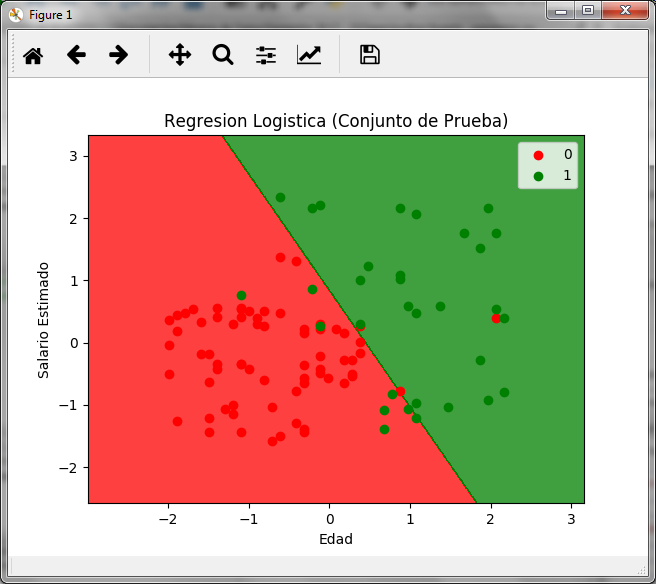
In the graph we can see the two regions, red for customers who do not buy with the value of y = 0 and green for customers who buy with the value of y = 1, in it we can also see the 8 green points on the red zone and the 3 red points on the green zone.

Dado que de 100 registros del conjunto de prueba 11 fueron clasificados erróneamente, podemos concluir que para este caso, la precisión del  modelo es del 89%

#the accuracy of the model is obtained with the score
score_test = classifier.score (X_test, y_test)

The value of the variable score_test is 0.89000, which means 89% accuracy in the classification and / or prediction.