Pre-processing of data
Nowadays we have a large amount of data generated by different sources and it becomes increasingly necessary to be able to analyze them in order to automatically extract all the information intelligence contained in them.
The specialized techniques focused on analysis of data, constitute both statistical methods and methods of artificial intelligence and machine learning, among others.
Ve este artículo en video
In this sense, the data mining in itself, it is a set of techniques aimed at discovering the information contained in large data sets.
The word discovery is related to the fact that much of the valuable information is previously unknown, it is about analyzing behaviors, patterns, trends, partnerships and other characteristics of the knowledge immersed in the data.
The process of data analysis or data science consists of several phases:
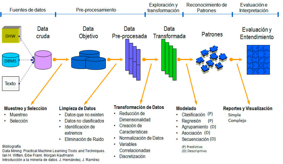
Pre-processing is a standardization of data prior to analysis model and this in turn consists of several phases as seen in the previous figure.
The Selection, Exploration, Cleaning and Transformation phases make up the pre-processing of the data necessary in many occasions, before applying any model of data analysis, either predictive or descriptive.
Sampling and Selection
In the selection phase, the relevant variables in the data are identified and selected, the variables that will provide us with the information for the subject in which we are working, as well as the sources that may be useful. Once the variables have been selected, appropriate sampling techniques are applied in order to obtain a sample of the data that is sufficiently representative of the population.
The sample allows inferring the properties or characteristics of the entire population with a error Measurable and measurable.
From the sample, the population characteristics (mean, total, proportion, etc.) are estimated with a quantifiable and controllable error.
The errors are quantified by means of the variance, the standard deviation or the calculation of the mean square error to obtain the accuracy of the errors.
It is important to take into account that to obtain the degree of representativeness of the sample it is necessary to use probabilistic sampling.
Exploration
Since the data come from different sources, it is necessary to explore them using techniques of exploratory analysis to identify unusual values, extreme values, missing values, discontinuities or other peculiarities of them.
With this, the exploration phase helps determine if the techniques of analysis of data that are taken into consideration. Therefore, it is necessary to carry out a preliminary analysis of the information available before the use of any technique.
We must examine the individual variables and the relationships between them, as well as evaluate and solve problems in the design of research and data collection.
The exploration may indicate the need to transform the data if the technique needs a normal distribution or if nonparametric tests are needed.
Exploratory analysis includes formal techniques and graphic or visual techniques
Cleaning
Since in the data set there may be outliers, missing values and / or erroneous values, cleaning them is important to solve some of these problems. This phase is a consequence of the exploratory analysis.
Transformation
The transformation of the data is necessary when there are different scales between the variables or there are too many or few variables, then normalization or standardization of the data is carried out by techniques of reduction or increase of the dimension, as well as simple or multidimensional scaling.
If the exploratory analysis indicates the need to transform some variables, some of these four transformations may be applied:
- Logical transformations
- Linear transformations
- Algebraic transformations
- Non-linear transformations
These phases mentioned in the previous points, constitute the process of pre-processing of the data and to apply these concepts, the following example is presented:
Pre-processing example
Suppose the following data table, which represents information from a store that linked data from customers who bought and customers who did not buy:
| Do not | country | Age | Salary | Purchase |
| 1 | France | 44 | 72000 | Do not |
| 2 | Spain | 27 | 48000 | Yes |
| 3 | Germany | 30 | 54000 | Do not |
| 4 | Spain | 38 | 61000 | Do not |
| 5 | Germany | 40 | Yes | |
| 6 | France | 35 | 58000 | Yes |
| 7 | Spain | 52000 | Do not | |
| 8 | France | 48 | 79000 | Yes |
| 9 | Germany | 50 | 83000 | Do not |
| 10 | France | 37 | 67000 | Yes |
As we can see, there are records with missing data. The client of the record or line 5 does not have salary and the client of line 7 does not have age.
When there are missing data, there are several strategies that can be followed, especially if the randomness of such missing data has been proven. One strategy is to use the method of approximation of complete cases which consists in including in the analysis only the cases with complete data, only rows whose values for all the variables are valid.
In this case we have to validate if the sample is affected or not by eliminating incomplete cases.
The alternative to data removal methods is the imputation of missing information, where the objective is to estimate the absent values based on valid values of other variables or cases.
One method to carry out the imputation of the missing information is the case substitution method. This consists in replacing the missing data with non-sample observations data, that is, they do not belong to the sample.
The substitution method by the mean or median, substitutes missing data for the value of the mean or median of all valid values of its corresponding variable. When there are extreme or atypical values, the missing data are replaced by the median, otherwise the average is used.
The imputation method by interpolation substitutes each missing value by the mean or median of a certain number of data or observations adjacent to it, especially when there is too much variability in the data. If there is no such variability, then they are replaced by the value resulting from an interpolation with the adjacent values.
Additionally, there is also the replacement method with a constant value and as its name indicates, the missing data are replaced by a constant value, valid for the variable in question, derived from external sources or from previous research.
Finally, we can also use the Imputation method by regression and this one uses the regression method to calculate or estimate the absent values based on their relationship with other variables in the data set.
In our example, we will use the mean as a value to impute the missing data of both age and salary. In this sense, the average age values are: 38.77 and for the salary, the average value of the values present in the sample is: 63,777.77, so the table is now as follows:
| Do not | country | Age | Salary | Purchase |
| 1 | France | 44 | 72000 | Do not |
| 2 | Spain | 27 | 48000 | Yes |
| 3 | Germany | 30 | 54000 | Do not |
| 4 | Spain | 38 | 61000 | Do not |
| 5 | Germany | 40 | 63777.77 | Yes |
| 6 | France | 35 | 58000 | Yes |
| 7 | Spain | 38.77 | 52000 | Do not |
| 8 | France | 48 | 79000 | Yes |
| 9 | Germany | 50 | 83000 | Do not |
| 10 | France | 37 | 67000 | Yes |
We already have the complete sample and now we continue with the categorical variables (Country and Purchase).
For the Buy variable, which has categorical values Yes or No, we can code it as 1 and 0 representing 1 for the value Si and 0 for the value No. For the case of the variable Country, the case is a little different since if we codify as 0, 1 and 2, the country with the value 2 would have more weight than the country with the value 0 so the strategy for this type of variables is different.
Within the logical transformations, interval variables can be converted into ordinals as the variables Talla or nominal as Color, and create dummy or dummy variables.
| country | France | Spain | Germany | |
| France | 1 | 0 | 0 | |
| Spain | 0 | 1 | 0 | |
| Germany | 0 | 0 | 1 |
The Country variable is changed by three variables (Dummy) that are the values of the Country variable. Instead of using the Country variable, we now use the 3 new variables and the table would look like this:
| Do not | France | Spain | Germany | Age | Salary | Purchase |
| 1 | 1 | 0 | 0 | 44 | 72000 | 0 |
| 2 | 0 | 1 | 0 | 27 | 48000 | 1 |
| 3 | 0 | 0 | 1 | 30 | 54000 | 0 |
| 4 | 0 | 1 | 0 | 38 | 61000 | 0 |
| 5 | 0 | 0 | 1 | 40 | 63777.77 | 1 |
| 6 | 1 | 0 | 0 | 35 | 58000 | 1 |
| 7 | 0 | 1 | 0 | 38.77 | 52000 | 0 |
| 8 | 1 | 0 | 0 | 48 | 79000 | 1 |
| 9 | 0 | 0 | 1 | 50 | 83000 | 0 |
| 10 | 1 | 0 | 0 | 37 | 67000 | 1 |
Given that the data of age and salary maintain a different scale and in the equations of the regression or some other method of classification and / or prediction, given the Euclidean distance between two points, the value of the salary could cause the age to stop be representative or important for the analysis, the most convenient is to make a scale transformation, be it a standardization or a normalization of the data.

For this example we will use normalization to adjust the scales of all the variables that is given by the current value of the sample minus the minimum value of the entire data set of that variable between the difference of the maximum value and the minimum value.
Once the normalization is applied, the resulting table is as follows:
| France | Germany | Spain | Age | Salary | Purchased |
| 1 | 0 | 0 | 0.72003861 | 0.71101283 | 0 |
| 0 | 0 | 1 | -1.62356783 | -1.36437577 | 1 |
| 0 | 1 | 0 | -1.20999022 | -0.84552862 | 0 |
| 0 | 0 | 1 | -0.1071166 | -0.24020695 | 0 |
| 0 | 1 | 0 | 0.1686018 | -6.0532E-07 | 1 |
| 1 | 0 | 0 | -0.52069421 | -0.49963052 | 1 |
| 0 | 0 | 1 | -0.00096501 | -1.01847767 | 0 |
| 1 | 0 | 0 | 1.27147542 | 1.3163345 | 1 |
| 0 | 1 | 0 | 1.54719383 | 1.6622326 | 0 |
| 1 | 0 | 0 | -0.2449758 | 0.2786402 | 1 |
When the categorical variables generate many dummy variables we can use the techniques of dimension reduction to make our data set more manageable.
Pre-processing with Python
Using python to perform the pre-processing of the previous example, it becomes easy with the numpy and sklearn libraries since the preprocessing subpackage contains the classes necessary to perform the imputation of missing data, the coding of the categorical variables, the creation of dummy variables and the adjustment of scales.
The first step is to import the libraries that we are going to use in processing, then we load the data set and store it in the dataset variable, we divide the matrix in x (independent variables) and Y (dependent variable)
# Pre-processing of data
import numpy ace np
import matplotlib.pyplot ace plt
import pandas ace P.S

# We load the data set
dataset = pd.read_csv ('Preproc_Datos_Compras.csv')
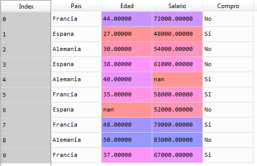
The loaded dataset is as follows and as we can see, the missing data is shown as nan (not a number):
Now we divide the variables into dependent and independent
# Pre-processing of data
import numpy ace np
import matplotlib.pyplot ace plt
import pandas ace P.S

# We load the data set
dataset = pd.read_csv ('Preproc_Datos_Compras.csv')

# We separate dependent and independent variables
x = dataset.iloc [:,:-1] y = dataset.iloc [:, 3]
When executing this last piece of code we have the variables x and y
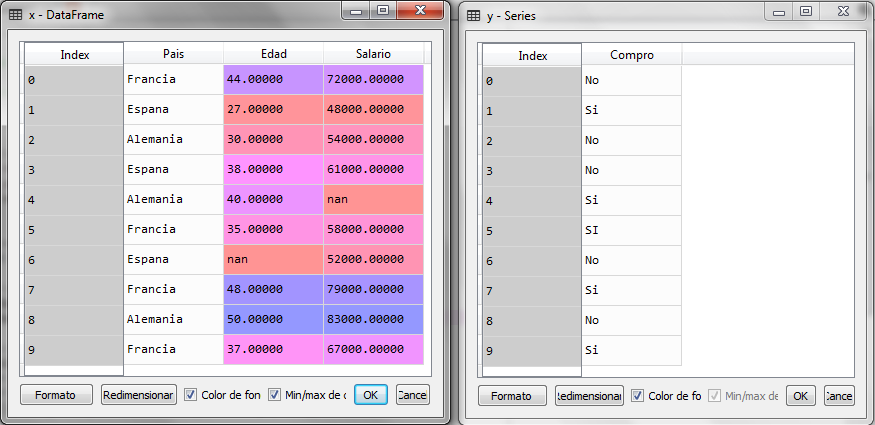
We see that in the matrix x, the missing data is shown as nan (Not an Object). The next step now is the imputation of the missing data and for this, we can use the Imputer class of the preprocessing subpackage.
# Pre-processing of data import numpy ace np import matplotlib.pyplot ace plt import pandas ace P.S # We load the data set dataset = pd.read_csv ('Preproc_Datos_Compras.csv') # We separate dependent and independent variables x = dataset.iloc [:,:-1] y = dataset.iloc [:, 3] #Imputation of missing data desde sklearn.preprocessing import Imputer imputer = Imputer (missing_values = 'NaN', strategy ='mean', axis =0) imputer = imputer.fit (x.values [:, 1:3]) x.iloc [:, 1:3] = imputer.transform (x.values [:, 1:3])
Once the fragment of the code of the Imputer class was executed, we observed that the missing data were calculated with the mean, which is the strategy that was indicated in the arguments of the constructor of the Imputer class.
The average value of the age was 38.77778 and the average value of the salary was 63.777.77778. The next step is the coding of the categorical variables. First we will do it for Y, with the values Yes and No and later for X with the values of the countries.
# Pre-processing of data import numpy ace np import matplotlib.pyplot ace plt import pandas ace P.S # We load the data set dataset = pd.read_csv ('Preproc_Datos_Compras.csv') # We separate dependent and independent variables x = dataset.iloc [:,:-1] y = dataset.iloc [:, 3] #Imputation of missing data desde sklearn.preprocessing import Imputer imputer = Imputer (missing_values = 'NaN', strategy ='mean', axis =0) imputer = imputer.fit (x.values [:, 1:3]) x.iloc [:, 1:3] = imputer.transform (x.values [:, 1:3]) # Coding of categorical variables desde sklearn.preprocessing import LabelEncoder label_encoder_y = LabelEncoder () y = label_encoder_y.fit_transform (y) label_encoder_x = LabelEncoder () x.iloc [:, 0] = label_encoder_x.fit_transform (x.values [:, 0]) desde sklearn.preprocessing import OneHotEncoder onehotencoder = OneHotEncoder (categorical_features = [0]) x = onehotencoder.fit_transform (x) .toarray ()
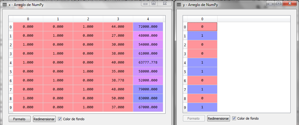
The LabelEncoder class encodes the values of Y in 0 for No and 1 for Yes, for the countries it codes them in 0 France, 1 Spain and 2 Germany, afterwards the OneHotEncoder classes performs the transformation of the dummy variables being as follows:
Finally, we only need the transformation of scales for the variables of Age and Salary.
# Pre-processing of data import numpy ace np import matplotlib.pyplot ace plt import pandas ace P.S # We load the data set dataset = pd.read_csv ('Preproc_Datos_Compras.csv') # We separate dependent and independent variables x = dataset.iloc [:,:-1] y = dataset.iloc [:, 3] #Imputation of missing data desde sklearn.preprocessing import Imputer imputer = Imputer (missing_values = 'NaN', strategy ='mean', axis =0) imputer = imputer.fit (x.values [:, 1:3]) x.iloc [:, 1:3] = imputer.transform (x.values [:, 1:3]) # Coding of categorical variables desde sklearn.preprocessing import LabelEncoder label_encoder_y = LabelEncoder () y = label_encoder_y.fit_transform (y) label_encoder_x = LabelEncoder () x.iloc [:, 0] = label_encoder_x.fit_transform (x.values [:, 0]) desde sklearn.preprocessing import OneHotEncoder onehotencoder = OneHotEncoder (categorical_features = [0]) x = onehotencoder.fit_transform (x) .toarray () # Transforming scales desde sklearn.preprocessing import StandardScaler sc_x = StandardScaler () sc_y = StandardScaler () x = sc_x.fit_transform (x) y = sc_y.fit_transform (y.reshape (-1, 1))
We apply the transformation of scales for both the variables of the set X and for the dependent variable Y and we see that now the if is 1 and the is not -1 to standardize all the values of all the variables.
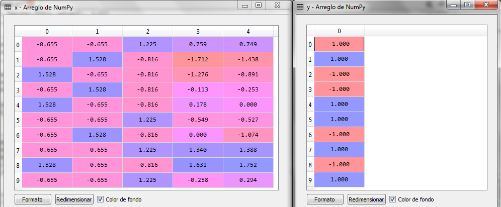
Now, with the pre-processed data we can apply some predictive method such as the Logistic Regression to predict the purchases of a new client, that is, with their data in country, age and salary, estimate whether to buy or not.
Ve este artículo en video
In the following articles we will present classification and prediction methods.
If you are interested in going deeper into these topics, we have the course of Python for Data Science, check here the details
Another very interesting course to start with python you can see here
For the basics of programming, we recommend the following course: Introduction to programming
On the other hand, to know the details to use cloud services with AWS, this course on Associate certification It is highly recommended, as well as the course of professional certification.
Finally in this webinar you will see the details to implement machine learning techniques in Azure
Subscribe to the blog to receive notifications when new articles are added


As always, with everything, true teacher. I'm Sergio López, from TESE, regards
Thank you very much Sergio
Te agradezco por este tutorial es Excelente y mu práctico de seguir
Muchisimas gracias Fernando
Buenas noches Jacob, muy bueno el tutorial, una consulta adicional en caso una de las variables originales tenga valores negativos y positivos, se puede aplicar también la estandarización o hay algun método adicional?. Gracias!!!
Gracias por el tutorial Jacob, una consulta adicional, en caso la variable original tenga valores negativos y positivos también se puede aplicar estandarización, o es recomendable algún otro método?. Saludos
Si, no importa el signo. De hecho en la estandarización o normalización el resultado arroja también números negativos.
Hola,
Si, no hay problema con los números negativos, la estandarización se puede usar, al igual que la normalización. El problema sería si existieran valores atípicos. Por que los mínimos, máximos y la media cambian radicalmente. Pero con valores negativos no sucede.